

Table of contents 

- Introduction -- Types of connections
- Overall view of basic connections
- Granger Causality
- Cross-convergent mapping (CCM)
- Dimensional causality
- Summary
$\textit{Kristóf Furuglyás, Theoretical Physics Seminar, 2019 Fall }$
About Causality 
- Having two discrete time series $X$ and $Y$
- One would like to infer the relation between them
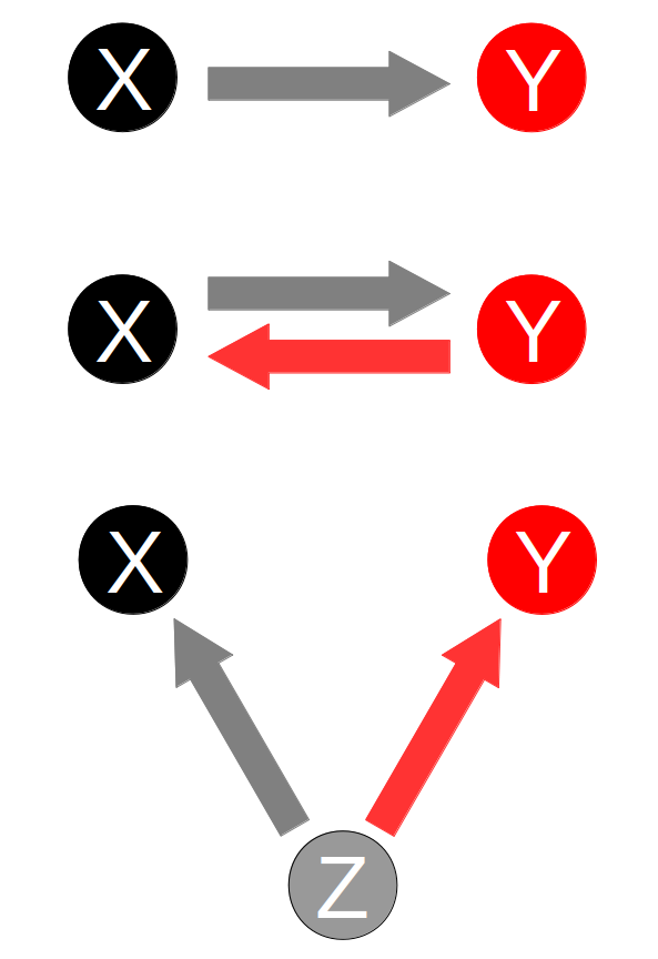
- Types of connections:
- Independent $X \perp Y$
- Unidirectional $X\rightarrow Y$ or $X\leftarrow Y$
- Bidirectional $X \leftrightarrows Y$
- (Hidden) Common cause $X \Lsh \Rsh Y $
- Last not explored yet totally
$\textit{Kristóf Furuglyás, Theoretical Physics Seminar, 2019 Fall }$
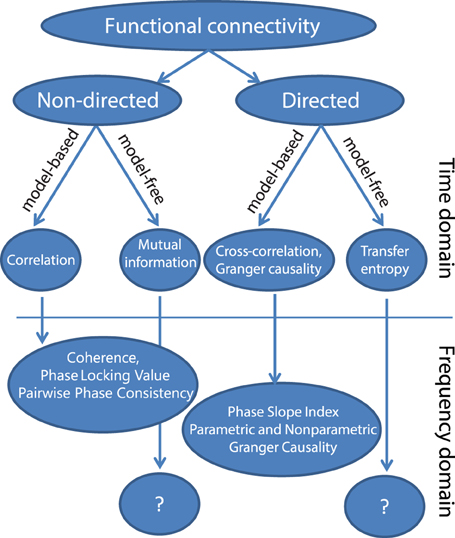
Taxonomy of connectivity 
$\textit{Kristóf Furuglyás, Theoretical Physics Seminar, 2019 Fall }$
Examples 
plots, labels = array([A, B, C, D]), ["A", "B = A+$\pi/6$", "C = A+$\pi/2$","D = Const."]
plt.title("Signals (Fs = 8kHz, f = 5 Hz)")
plt.plot(x, plots.T)
plt.grid()
plt.legend(labels, loc = 'best')
plt.xlabel('Time (s)')
plt.ylabel('Signal');

Simpler connections in time domain 
- Pearson correlation (non-directed, model-based): $$ r_{xy}=\frac {\sum _{i=1}^{n}(x_{i}-{\bar {x}})(y_{i}-{\bar {y}})}{{\sqrt {\sum _{i=1}^{n}(x_{i}-{\bar {x}})^{2}}}{\sqrt {\sum _{i=1}^{n}(y_{i}-{\bar {y}})^{2}}}} $$
print("Pearson correlation| A-B:", round(pearsonr(A,B)[0],4), "A-C:",
      round(pearsonr(A,C)[0],4), "A-D:", round(pearsonr(A,D)[0],4))
- Mutual information (non-directed, model-free): $$ I(X;Y) = \sum_{x,y} P_{XY}(x,y) \log {P_{XY}(x,y) \over P_X(x) P_Y(y)} = E_{P_{XY}} \log{P_{XY} \over P_X P_Y} $$
print("The entropies|       A: ", round(entropy1(A),4), " B: ",
      round(entropy1(B),4), " C: ", round(entropy1(C),4), " D: ", round(entropy1(D),4))
print("Mutual information| A-B:", round(mutual_info_score(A, B),4), "A-C:",
      round(mutual_info_score(A,C),4), "A-D:", round(mutual_info_score(A,D),4))
print("As a reference|     A-A:", round(mutual_info_score(A,A),4), "B-B:",
      round(mutual_info_score(B,B),4), "C-C:", round(mutual_info_score(C,C),4))
- Cross correlation (directed, model-based):
grid()
plot(correlate(A,B))
plot(correlate(A,C))
plot(correlate(A,D))
legend(["A-B", "A-C", "A-D" ], loc = 'best')
xlabel('Data point');

$\textit{Kristóf Furuglyás, Theoretical Physics Seminar, 2019 Fall }$
- Transfer entropy (directed, model-free):
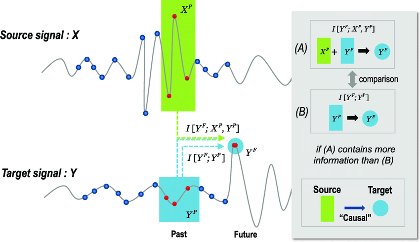
$\textit{Kristóf Furuglyás, Theoretical Physics Seminar, 2019 Fall }$
Frequency domain 
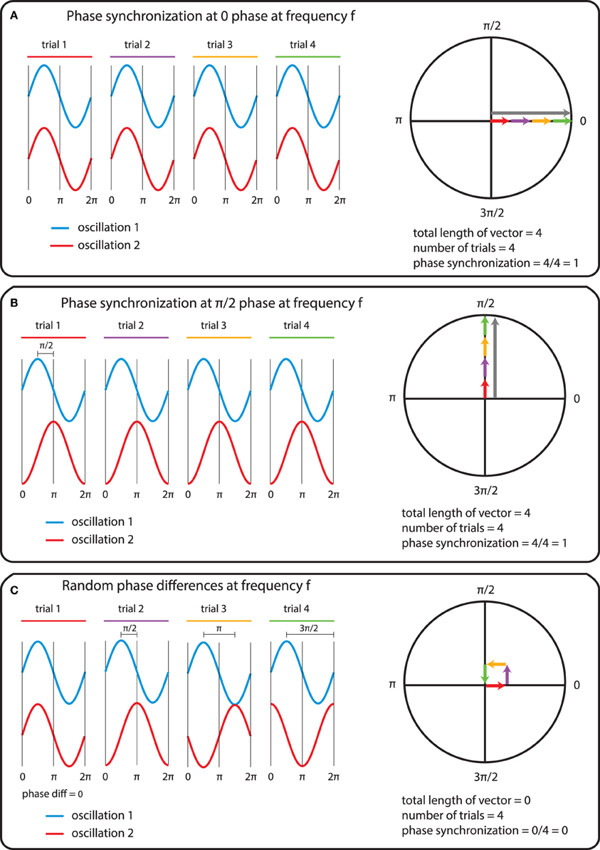
- Coherence $$ \gamma _{xy}^{2}(f)={\frac {|S_{xy}(f)|^{2}}{S_{xx}(f)S_{yy}(f)}} $$
plt.plot(x, array([A,B]).T)
plt.xlim(0.4, 0.42)
plt.grid()
plt.xlabel("Time [sec]")
plt.ylabel("Signal")
plt.legend(["A (1kHz)", "A + B (1.5kHz) + noise"], loc = "best");

plt.semilogy(f,c)
plt.grid()
plt.xlabel("Frequency [Hz]")
plt.ylabel("Coherence");

$\textit{Kristóf Furuglyás, Theoretical Physics Seminar, 2019 Fall }$
 - Phase Slope Index (PSI) - by Nolte et al. (2008) :
$$
\tilde{\Psi}_{ij} = \Im \left( \sum_f C_{ij}^* \left( f \right) C_{ij} \left( f + \delta f \right)\right)
$$
- Phase Slope Index (PSI) - by Nolte et al. (2008) :
$$
\tilde{\Psi}_{ij} = \Im \left( \sum_f C_{ij}^* \left( f \right) C_{ij} \left( f + \delta f \right)\right)
$$
$\textit{Kristóf Furuglyás, Theoretical Physics Seminar, 2019 Fall }$
Granger causality 
$$ x\left[t\right] = \sum^m_{i=1} a_i x\left[t-i \right] + \epsilon_1 \text{ and } y\left[t\right] = \sum^m_{i=1} b_i y\left[t-i \right] + \epsilon_2 $$
$$ x\left[t\right] = \sum^m_{i=1} c_i x\left[t-i \right] + \sum^q_{i=1} d_i y\left[t-i \right] + \epsilon_3 $$ $$y\left[t\right] = \sum^m_{i=1} e_i x\left[t-i \right] + \sum^q_{i=1} f_i y\left[t-i \right] + \epsilon_4 $$
$\textit{Kristóf Furuglyás, Theoretical Physics Seminar, 2019 Fall }$
Granger Causality 
$$ F_{y\rightarrow x} = \ln \left(\frac{var\left( \epsilon_1\right)}{var\left( \epsilon_3\right)} \right) \text{ and } F_{x\rightarrow y} = \ln \left(\frac{var\left( \epsilon_2\right)}{var\left( \epsilon_4\right)} \right) $$
$$ F_{y\rightarrow x} = \ln \left(\frac{\frac{var\left( \epsilon_1\right) - var\left( \epsilon_3\right)}{m}}{\frac{var\left( \epsilon_3\right)}{T-2m-1}} \right) $$
$\textit{Kristóf Furuglyás, Theoretical Physics Seminar, 2019 Fall }$
Problems with Granger causality 
As George Sugihara mentioned (Sugihara et al. (2012)):
However, as Granger realized early on, this approach may be problematic in deterministic settings, especially in dynamic systems with weak to moderate coupling. [...]
That is to say, in deterministic dynamic systems (even noisy ones), if X is a cause for Y, information about X will be redundantly present in Y itself and cannot formally be removed from U—a consequence of Takens’ theorem.
$\textit{Kristóf Furuglyás, Theoretical Physics Seminar, 2019 Fall }$
Cross-cenvergent mapping 
- A method invented by Sugihara et al., 2012 to infer weakly coupled causalities based on their joint manifold.
- Promising for circular causality and nonlinear coupling.
- Taken's theorem: provides the conditions under which a smooth attractor can be reconstructed from the observations made with a generic function. [...] The reconstruction preserves the properties of the dynamical system that do not change under smooth coordinate changes (i.e., diffeomorphisms), but it does not preserve the geometric shape of structures in phase space.
$\textit{Kristóf Furuglyás, Theoretical Physics Seminar, 2019 Fall }$
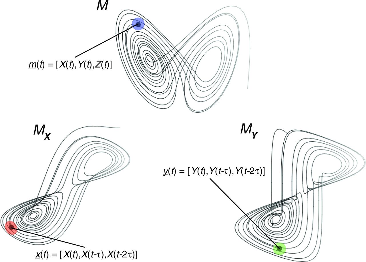
Embedding 
- The trajectory reconstructed in the state space is topologically equivalent With the trajectory of the system's original trajectory in its real space.
- Points that are neighbors in the state-space of the consequence should be neighbors in the state space of the cause as well.
- This topology preserving property can be tested by the cross mapping method.
$\textit{Kristóf Furuglyás, Theoretical Physics Seminar, 2019 Fall }$
Embedding 
$${\begin{aligned}{\frac {\mathrm {d} X}{\mathrm {d} t}}&=\sigma (Y-X),\\[6pt]{\frac {\mathrm {d} Y}{\mathrm {d} t}}&=X(\rho -Z)-Y,\\[6pt]{\frac {\mathrm {d} Z}{\mathrm {d} t}}&=XY-\beta Z.\end{aligned}}$$
$\textit{Kristóf Furuglyás, Theoretical Physics Seminar, 2019 Fall }$
Short introduction about CCM 
$\textit{Kristóf Furuglyás, Theoretical Physics Seminar, 2019 Fall }$
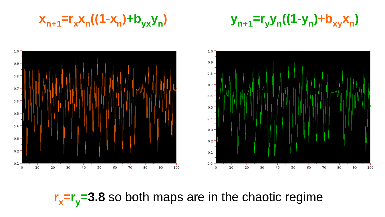
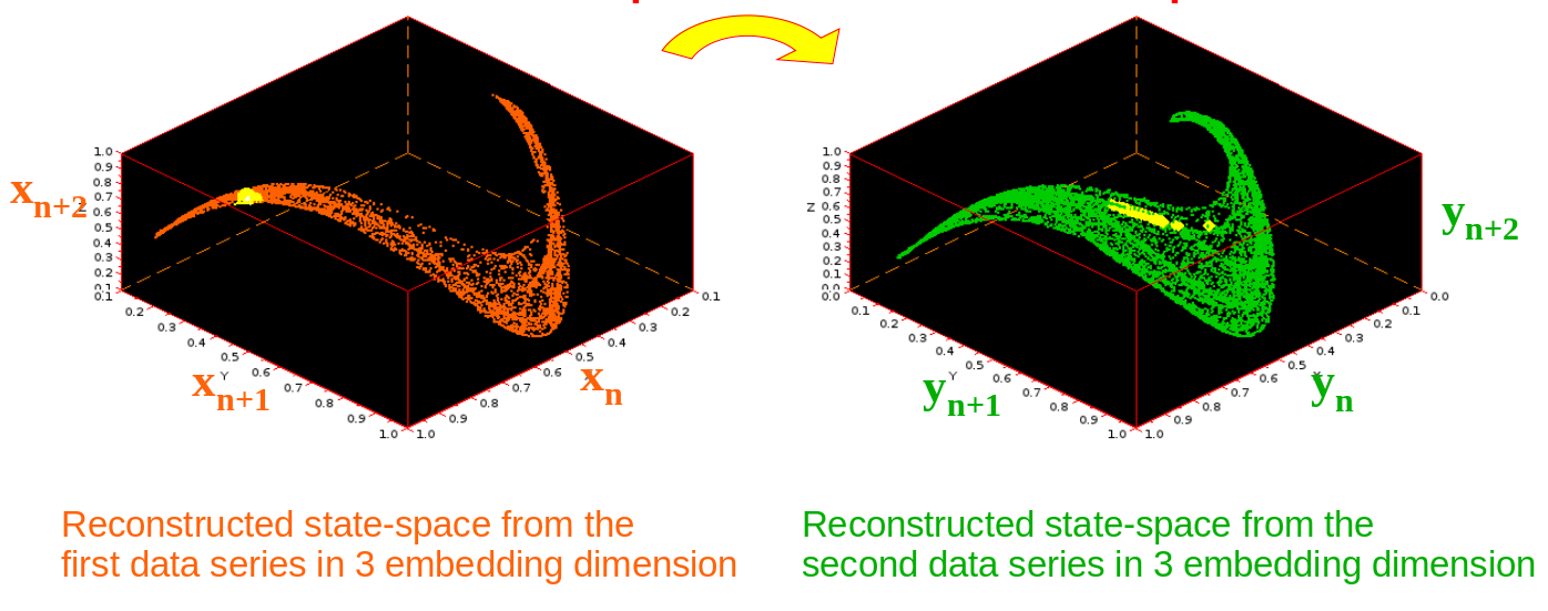
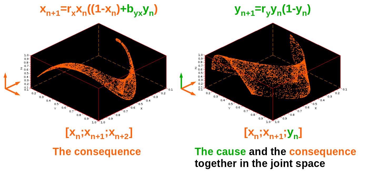
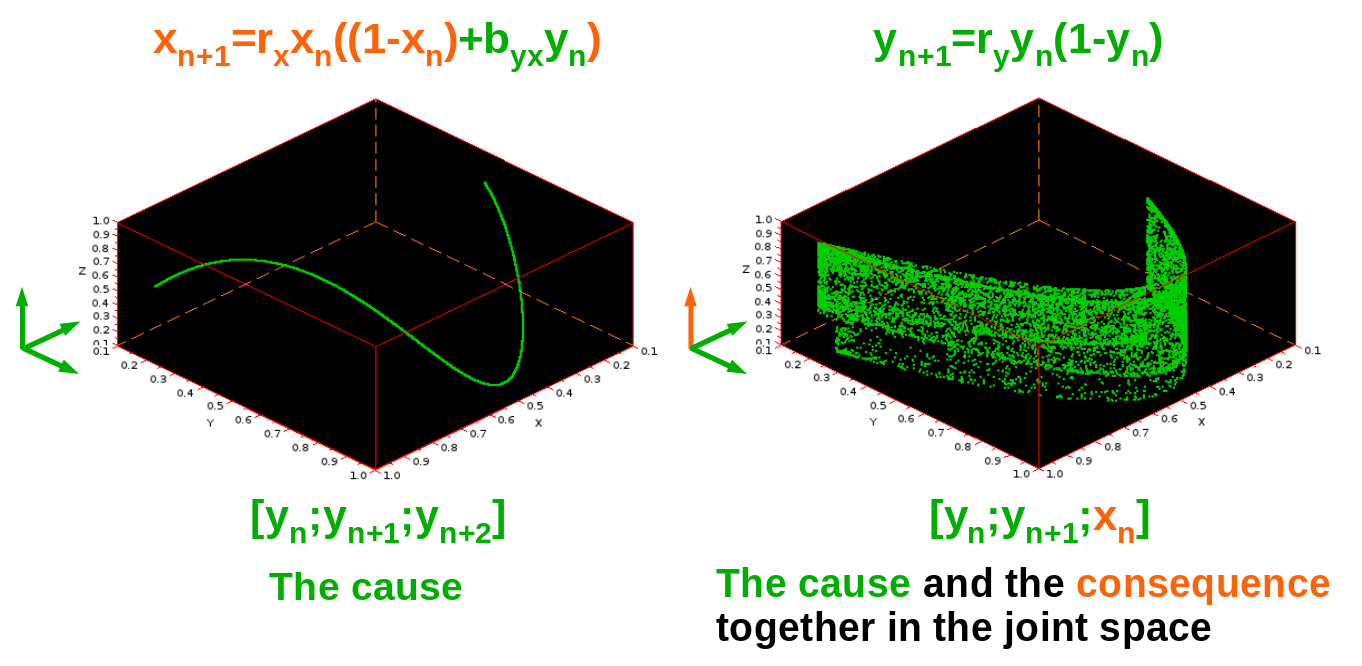
CCM on logistic maps 
$\textit{Kristóf Furuglyás, Theoretical Physics Seminar, 2019 Fall }$
CCM on logistic maps 
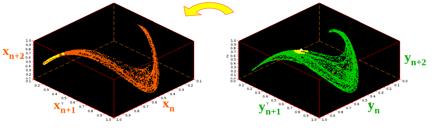
$\textit{Kristóf Furuglyás, Theoretical Physics Seminar, 2019 Fall }$
CCM on logistic maps 
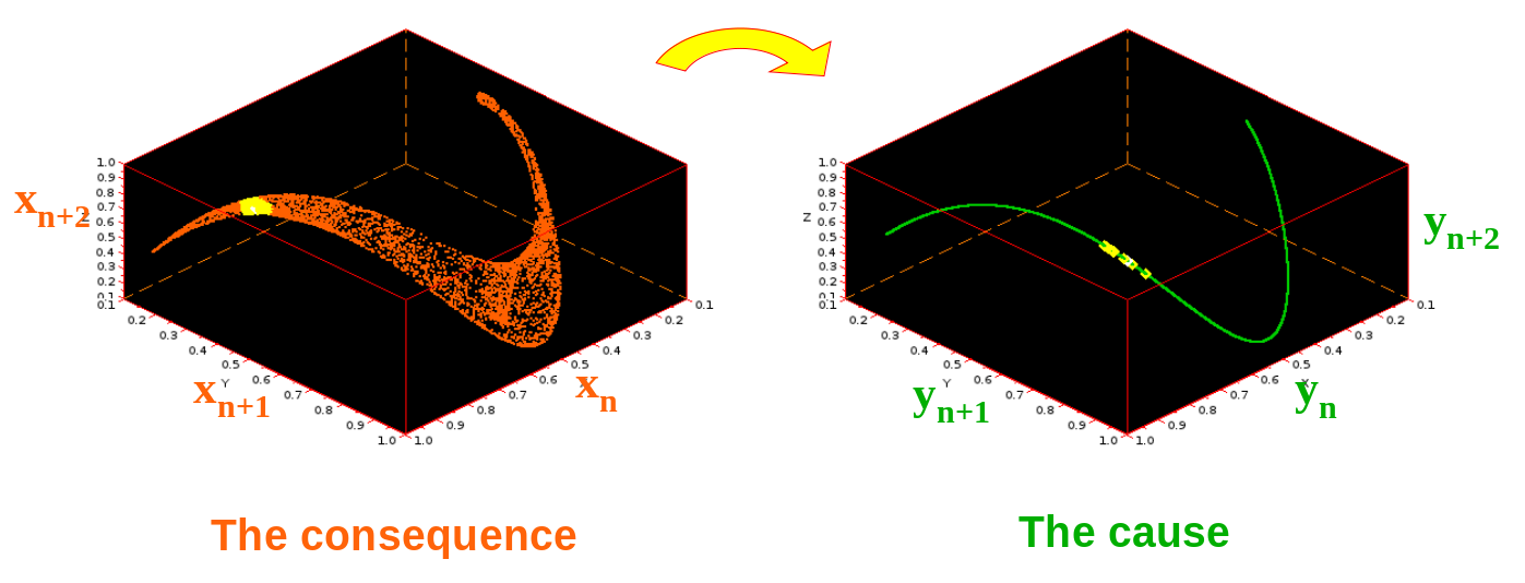
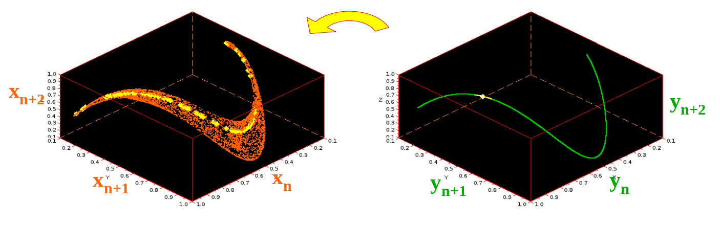
$\textit{Kristóf Furuglyás, Theoretical Physics Seminar, 2019 Fall }$
Time-delayed CCM 
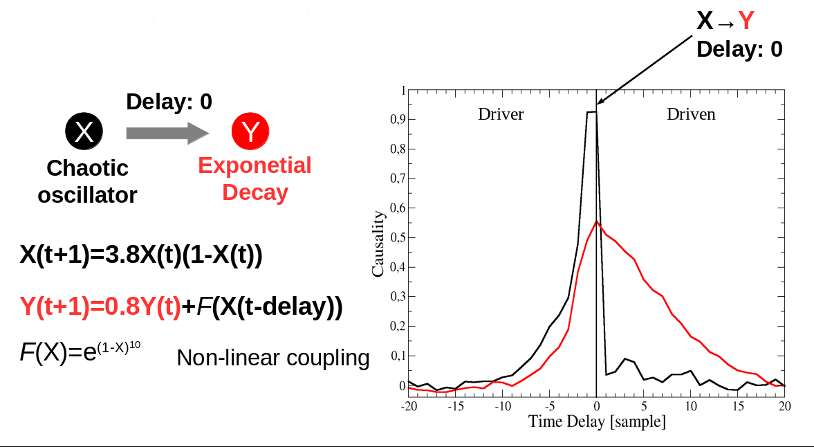
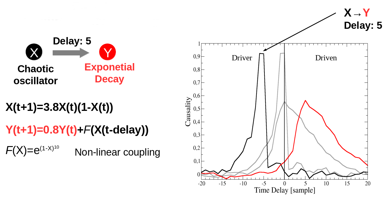
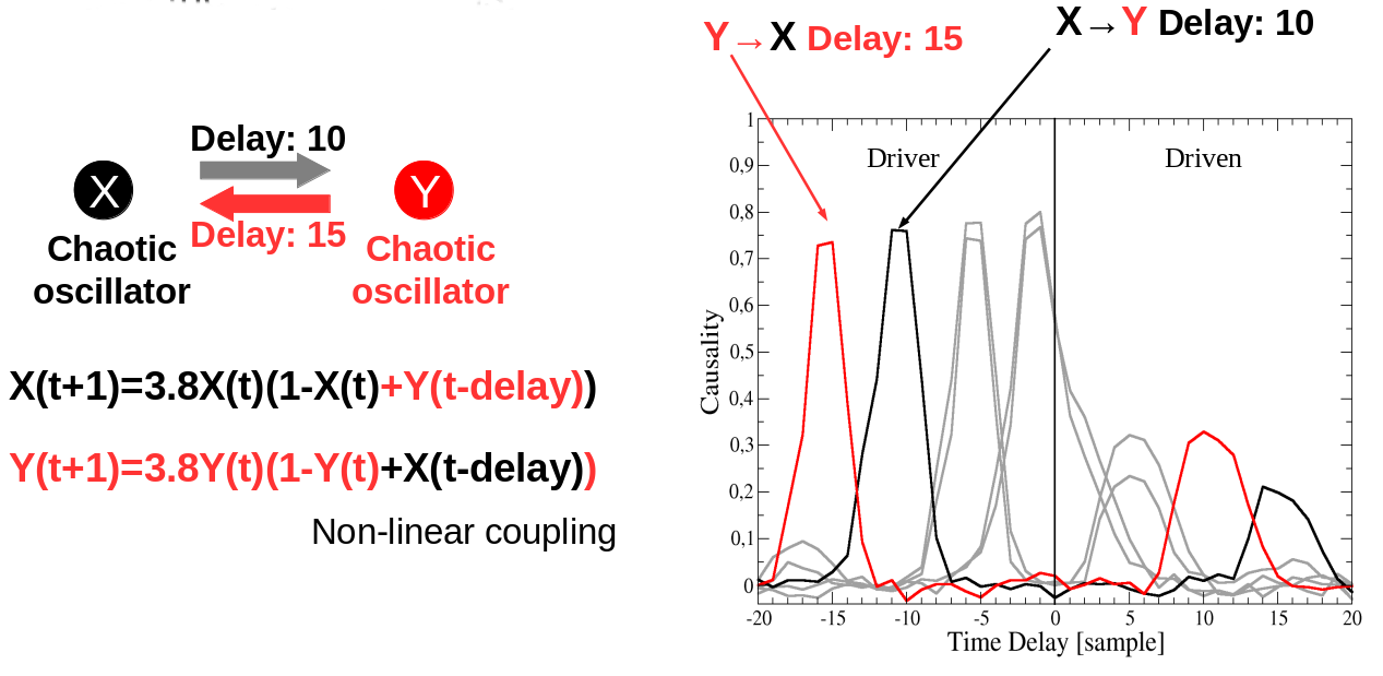
$\textit{Kristóf Furuglyás, Theoretical Physics Seminar, 2019 Fall }$
Time-delayed CCM 
- Even for the bidirectional case, many may fail to detect causality.
- Choosing the proper method is not exact.
- None of them can detect a hidden common cause.
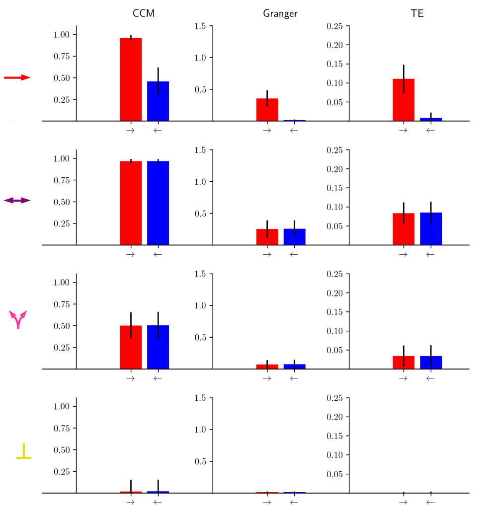
$\textit{Kristóf Furuglyás, Theoretical Physics Seminar, 2019 Fall }$
Dimensional causality 
- Method developed by Benkő et al. (2018) to detect the hidden common cause based on the dimensions of the fractals created in the joint space.
- Key point: the cause does not increases the dimension of the consequence in the joint space, the information is already there!
$\textit{Kristóf Furuglyás, Theoretical Physics Seminar, 2019 Fall }$
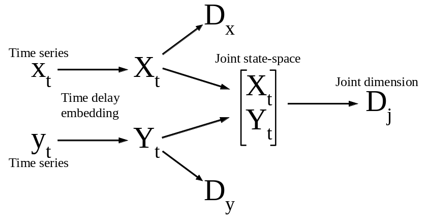
Mathematical approach 
Information dimension introduced by Rényi (1959): $$ d_X = \lim_{N\rightarrow\infty} \frac{1}{\log N} H\left( \left[X\right]_N\right), $$
Since $X$ is discrete and finite, if the variable lives in a $D$ dimensional space, a proper estimate needs at least $10^D-30^D$ sample points. An approximate form :
$$ d_{X, 1/N} = \frac{1}{\log N} H\left( \left[X\right]_N\right). $$Assumption 1: time series are stationary. Local intrinsic dimenson:
$$ D_X\left(x\right) = \lim_{r\rightarrow 0} \frac{1}{\log r} \log P \left( X \in B\left(x,r \right)\right), $$The intrinsic dimension:
$$ d_X = D_X = E\left( D_X\left( X \right) \right) $$$\textit{Kristóf Furuglyás, Theoretical Physics Seminar, 2019 Fall }$
Mathematical approach 
Assumption 2: the embedded manifolds are homogeneous with respect to (the existing) dimension. Local intrinsic dimension estimates:
$$ \hat{D} \left(x \right)_r = \frac{1}{\log r} \log \left| N \left(x,r \right) \right|. $$Global dimension estimate:
$$ \hat{D}_{X,r} = \frac{1}{n} \sum_{i=1}^n \hat{D} \left(x_i \right)_r $$For the $k$-th nearest neighbour, one shall calculate the dimension from the distance $r(x,k) = d(x, X^k(x))$. In this setting, the resolution is:
$$ r^D \approx \frac{k}{n} $$$\textit{Kristóf Furuglyás, Theoretical Physics Seminar, 2019 Fall }$
Detection of causality 
- Independent
$$X \perp Y \Rightarrow D_J = D_X + D_Y$$
- Unidirectional
$$X\rightarrow Y \Rightarrow D_J = D_Y <D_X + D_Y $$
- Bidirectional
$$X \leftrightarrows Y \Rightarrow D_J = D_X = D_Y$$
- (Hidden) Common cause $$X \Lsh \Rsh Y \Rightarrow \max\left(D_X, D_Y \right) < D_J < D_X + D_Y$$
$\textit{Kristóf Furuglyás, Theoretical Physics Seminar, 2019 Fall }$
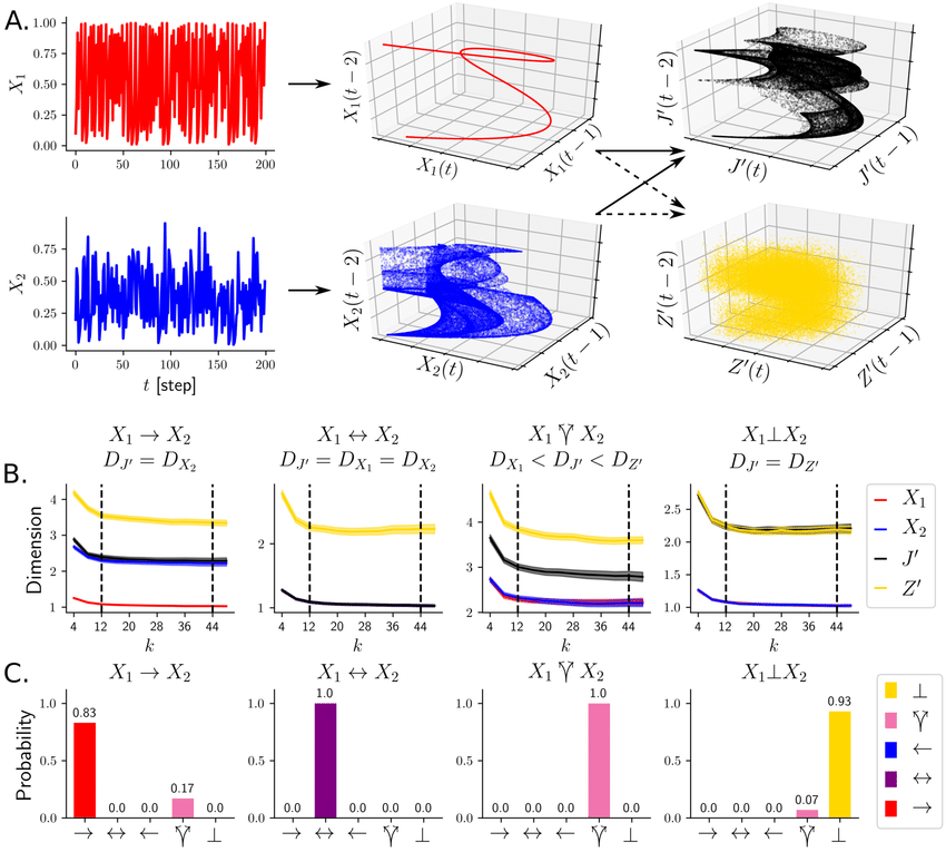
Testing on logistic maps 
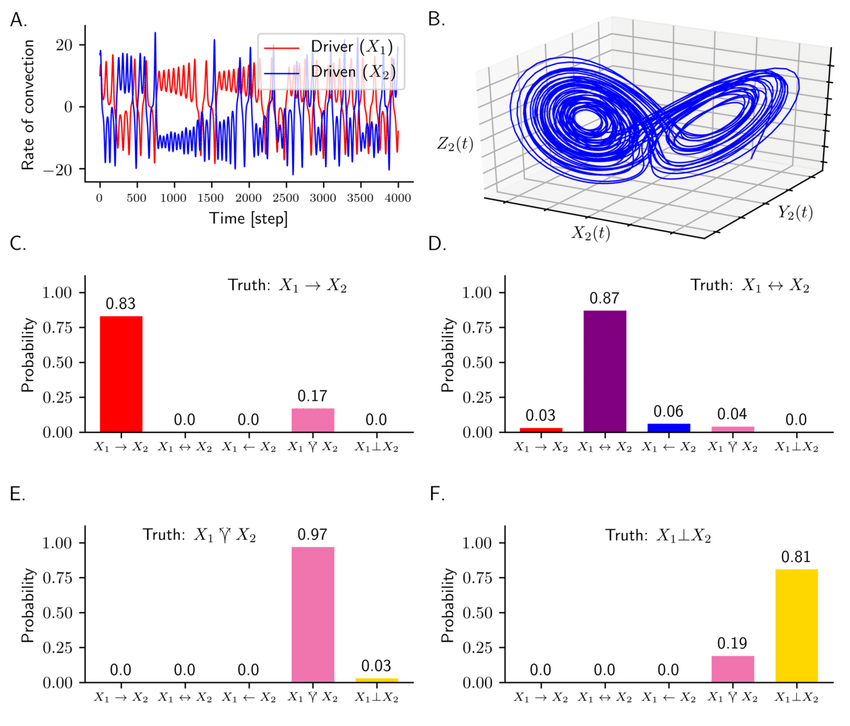
Testing on Lorenz systems 
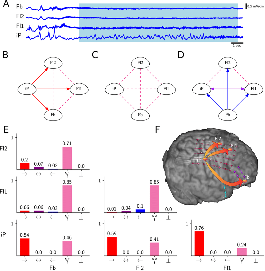
Real world example 
Summary 
- Investigated connectivity types and their measures,
- Explored Granger causality,
- Cross convergent mapping (with time delay),
- Introduced dimensional causality.
Further perspectives 
- Test DC for more time series from the real world,
- Optimize the dimension measurement,
- Explore more complex weakly coupled systems.
$\textit{Kristóf Furuglyás, Theoretical Physics Seminar, 2019 Fall }$
References 
- Bastos, André M., and Jan-Mathijs Schoffelen. "A tutorial review of functional connectivity analysis methods and their interpretational pitfalls." Frontiers in systems neuroscience 9 (2016): 175.
- P. Wollstadt, J. T. Lizier, R. Vicente, C. Finn, M. Martinez-Zarzuela, P. Mediano, L. Novelli, M. Wibral (2018). IDTxl: The Information Dynamics Toolkit xl: a Python package for the efficient analysis of multivariate information dynamics in networks. ArXiv preprint: https://arxiv.org/abs/1807.10459.
- Lee, Uncheol & Ku, Seungwoo & Noh, Gyujeong & Baek, Seunghye & Choi, Byung-Moon & Mashour, George. (2013). Disruption of Frontal-Parietal Communication by Ketamine, Propofol, and Sevoflurane. Anesthesiology. 118. 1264-1275. 10.1097/ALN.0b013e31829103f5.
- Nolte, Guido, et al. "Comparison of granger causality and phase slope index." Causality: Objectives and Assessment. 2010.
- Granger, Clive WJ. "Investigating causal relations by econometric models and cross-spectral methods." Econometrica: Journal of the Econometric Society (1969): 424-438.
- Sugihara, G., May, R., Ye, H., Hsieh, C. H., Deyle, E., Fogarty, M., & Munch, S. (2012). Detecting causality in complex ecosystems. science, 338(6106), 496-500.
- Benkő, Z., Zlatniczki, A., Fabó, D., Sólyom, A., Erőss, L., Telcs, A., & Somogyvári, Z. (2018). Exact Inference of Causal Relations in Dynamical Systems. arXiv preprint arXiv:1808.10806.
- Renyi, A. On the dimension and entropy of probability distributions. Acta Mathematica Academiae Scientiarum Hungarica 10, 193–215(1959).